Modern and Advanced Kelvin Probe Force Microscopy (KPFM)

Kelvin probe force microscopy (KPFM) is a key electrical mode used in scanning probe microscopy. It measures a fundamental physical property of materials – a surface potential. Compared to other modes, where the extraction of quantitative data is subject to a variety of usually complex calibration routines, quantification of a KPFM measurement is generally straightforward as the difference between the surface potentials of a scanning probe and the sample is measured in volts. This voltage is commonly known as a contact potential difference (CPD). Where metals are concerned, it is equal to the difference in work functions between the tip and the sample materials.

The work function is of significant importance concerning the study of semiconductor materials, the chemistry of fuel cells, photovoltaics of solar cells, lithium battery research, properties of alloys, conducting polymers, material differentiation in composite compounds, 2D materials, and several other areas.¹

Initially, the wide adoption of conventional KPFM was slow, due to the lack of spatial resolution and topography artifacts. However, innovative KPFM methods have pushed these limits and demonstrated significant improvement in resolving smaller features. This, in turn, has made KPFM one of the leading electrical modes.

This article outlines the physics behind the KPFM technique and the difference between various modes, and provides measurement examples of a few standard samples. The measurements in this article were made in single-pass mode.

Background

The method originates from an experiment measuring electrostatic forces between the plates of a parallel plate capacitor, made of various metals, first performed by Lord Kelvin.² A more recent interpretation of the CPD measurement was later realized by Walter Zisman.³

KPFM experiments were first carried out shortly after the atomic force microscope (AFM) was invented at Watson Research Center (IBM) by Weaver⁴ and Nonnenmacher⁵ working at different labs.

In a KPFM measurement, the AFM probe is positioned just a short distance above the sample surface via the mechanical feedback loop (Figure 1). The KPFM controller applies an AC voltage between the tip and the sample, generating an electrostatic AC force, and reducing this force automatically by applying the bucking DC voltage.

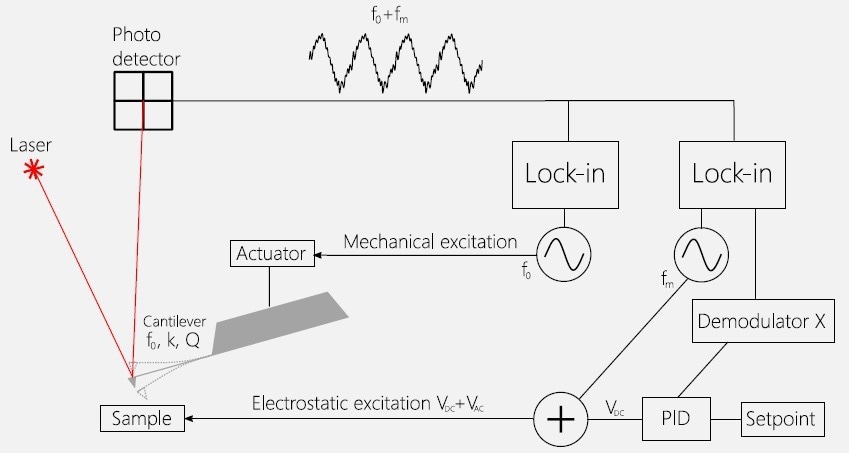
 Figure 1. Principles of Kelvin probe force microscopy. A cantilever with a resonant frequency f₀, spring constant k and quality factor Q is mechanically excited at its resonant frequency by an oscillator. The AC signal on the photodetector on that frequency is detected by a lock-in amplifier and is used for the topography measurement and the control of the cantilever position above the sample. This is a so-called mechanical loop. Another oscillator is set to modulate the sample potential on a modulation frequency f_m. The electrical AC excitation is added to a DC bias voltage, and this V_AC + V_DC potential is applied to the sample. The AC electrostatic interaction between the sample and the cantilever depends on the value of the V_DC. A PID controller is set to zero this interaction (the value of the Demodulator X) by adjusting the value of the V_DC. When the electrostatic interaction between the tip and the sample is zero, both are at the same potential, and the value of V_DC would be the contact potential difference or (CPD). Image Credit: Nanosurf AG

Both AC and DC voltages can be applied to either the sample or the tip, while the other one (tip or sample) remains on the ground.

In practice, advanced KPFM controllers would have several lock-ins and an additional phase-locked loop (PLL).

The variation of the bucking voltage while scanning the tip above the sample is recorded as an XY map of CPD. The most basic KPFM controller has at least one lock-in amplifier for the AC excitation and detection, and a PID controller to ensure the system can preserve a minimal response.

AM and FM KPFM

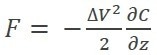
To better comprehend the basic physics of the KPFM, the force F coming from the electrostatic interaction should be considered when the AC voltage is applied between the tip and the sample (Eq. 1):

(4)

In this equation, DV represents the voltage between the tip and the sample, C is the tip-sample capacitance, and z represents the distance between them. The expression for the DV can be written as follows (Eq. 2):

where V_CPD is representative of the contact potential difference, and the V_DC and the V_AC are the bucking and the AC voltage, used by the KPFM controller.

When the ∆V is substituted in Eq. 1 for the expression in Eq. 2, the extended expression for the force can be shown as (Eq. 3):

(3)

The first two terms show no variance with time and are qualified as DC terms. The principle of the amplitude-modulated (AM) KPFM lies in the third term. The lock-in amplifier measures the amplitude and phase of the V_ACsin(ωt) signal, and the PID controller modifies the V_DC to offset this signal.

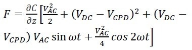
There are two slightly different ways to choose the working frequency for the electrostatic excitation: the first one is the application of the AC voltage at a frequency f_m far below the mechanical resonance of the tip f₀, and the second method includes applying this excitation at the frequency of the second mechanical eigenmode of the cantilever f₁ (Figure 2).

In the second instance, a better signal-to-noise ratio (SNR) is observed due to the extra amplification of the electrostatic signal by the mechanical resonator. In both cases of the AM-KPFM, the KPFM measures the electrostatic force, and the electrical excitation and detection are completed on the same frequency. The frequency-modulated (FM) KPFM, is dependent on the ∂C⁄∂z (or C’) part of Eq. 3.

When conducting a polynomial expansion of C’ and observing the first two members of the expansion, it can be shown⁶ that:

where a₀ is a constant, this effectively means that the C’ is dependent on the force gradient, as opposed to the force amplitude.⁶

This is the primary difference between AM and FM KPFM modes. There are numerous implementations of the FM KPFM, and the most prominent is heterodyne FM KPFM.

Heterodyne FM KPFM utilizes frequency mixing between the mechanical and the electrical excitations. The excitation frequency fm is selected to sit at the frequency difference between the second and the first mechanical eigenmodes of the cantilever: (f₁ – f₀).

In this instance, the mixed product will be placed at f₁, enabling mechanical amplification, as was necessary for AM KPFM on the 2^nd eigenmode (Figure 2). Due to the elevated excitation and detection frequencies, the heterodyne FM KPFM has greater bandwidth than the sideband AM KPFM.

Figure 2. Different KPFM implementations in a frequency domain. Black curves show mechanical motion of the cantilever, and black dotted lines show its mechanical excitation. Red dotted lines show electrical excitation and detection. (a) Off resonance AM KPFM. The electrical excitation f_m is done below the mechanical resonance of the cantilever f₀. Both excitation and detection are done on the same frequency. (b) AM KPFM at 2^nd eigenmode. The electrical excitation f_e is done above the mechanical resonance of the cantilever f₀ and at it’s 2^nd mechanical eigenmode f₁. Both excitation and detection are done on the same frequency. This mode's advantage is amplifying the electrostatic signal by a mechanical oscillator. (c) Heterodyne FM KPFM. The excitation frequency f_m = (f₁ - f₀) is chosen such, that the mixed product would fall directly on f₁. Because of higher excitation frequency, the heterodyne FM KPFM has much higher bandwidth than the AM KPFM. The second harmonics of the excitation and the mixed product carry information about the ∂C/∂z and ∂²C/∂²z.⁷. Image Credit: Nanosurf AG

Interaction Volume in AM and FM KPFM

The signal is proportional to the electrostatic force in AM KPFM. In FM KPFM, this is relevant to the force gradient. The result is that various parts of the AFM probe influence the contributions to the KPFM signal in AM and FM modes.

When in AM mode at tip-sample distances exceeding 1 nm, the signal is dominated by the cantilever part. When the signal is close to 1Å, the signal from the tip apex moves towards the one from the cantilever. This restricts the spatial resolution of the method, and the AM KPFM is renowned for its inept performance when measuring small samples.

In the FM mode, already at about 10 nm above the surface, the most dominant contributions are from the tip apex and the tip cone. At 1 Å, the signal is dominated by the one from the tip apex (Figure 3).⁸ Due to a larger interaction volume, the AM KPFM typically has a greater signal-to-noise ratio, but the lateral resolution is where it suffers.

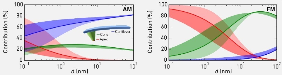
Figure 3. Comparison of contributions of different parts of the cantilever to the KPFM signal in AM and FM modes. In the AM KPFM mode, the signal is dominated by the interaction between the cantilever part of the AFM probe, and only at distances around 1 Å, the tip apex contribution becomes noticeable, but never exceeds the one from the cantilever. In the FM KPFM mode even at relatively large distances the main contribution comes from the tip cone and the tip apex, and at shorter distances, the signal if fully dominated by the tip apex contribution⁸. As a result, the AM KPFM has better signal-to-noise ratio, but the FM KPFM has better XY resolution and provides more credible measurement of VCPD. Image is taken from Ref 8. Image Credit: Nanosurf AG

On the other hand, FM KPFM has lower SNR and is better at resolving small features.

Cantilevers

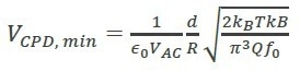
In earlier research surrounding KPFM, researchers experienced the limit to sensing the CPD voltage, which can be described as (Eq. 5):⁵

(5)

where the R = tip radius, d = tip-sample distance T = temperature, k = cantilever spring constant, Q = quality factor, B = bandwidth, f₀ = resonance frequency of the cantilever, k_B = Boltzmann constant, V_AC = amplitude of the AC voltage between the tip and the sample, and the ϵ₀ is the dielectric constant in a vacuum.

As this formula indicates, for the smallest detectable signal, a large tip radius, short distance to the sample, large AC voltage, and small sprint constant, are all requisite components. When it comes to selection, softer and shorter cantilevers are beneficial for the KPFM sensitivity, as well as applying larger AC amplitudes. However, larger AC amplitudes may cause reduced lateral resolution.

Experimental Comparison Between AM and FM KPFM

To fully demonstrate the differences between various KPFM modes, a series of typical KPFM samples were measured, followed by a comparison of the CPD signal and resolution in the captured images.

The first sample of interest is made up of aluminum dots on gold. Figure 4 displays the topography and the KPFM measurements with three different KPFM modes: the off-resonance AM KPFM, the AM KPFM on the 2^nd mechanical eigenmode, and the heterodyne FM KPFM.

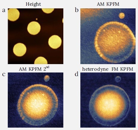
Figure 4. Comparison between the AM and FM KPFM modes on aluminum dots on gold sample. The image demonstrates the amplification of the KPFM signal between the AM KPFM on 2^nd eigenmode and the off-resonance AM KPFM. One can also see the topography signal mixing with the KPFM signal for both AM modes. The heterodyne KPFM is showing cleaner signal without topography cross-talk. (a) Image size: 20 x 20 μm², height range: 250 nm, (b) Image size: 7 x 7 μm², CPD range: 0.4 V, (c) Image size: 7 x 7 μm², CPD range: 0.45 V, (d) Image size: 7 x 7 μm², CPD range: 0.47 V. Image Credit: Nanosurf AG

The data indicates that the 2^nd eigenmode enhances the signal-to-noise ratio of the AM KPFM due to the amplification of the signal by the mechanical resonance. Both AM modes, however, reveal noticeable topography cross-talk – i.e. grains of metal visible in the surface potential.

Heterodyne FM KPFM is influenced to a lesser degree by this crosstalk. The second sample is the SRAM sample showing areas of p- and n-type doped silicon (Figure 5). Those are usually demonstrating good contrast in the KPFM. Again, the AM KPFM on the 2^nd mechanical resonance demonstrates an improvement in SNR. However, the FM KPFM shows a greater signal span on the signal cross-section and overall good image quality.

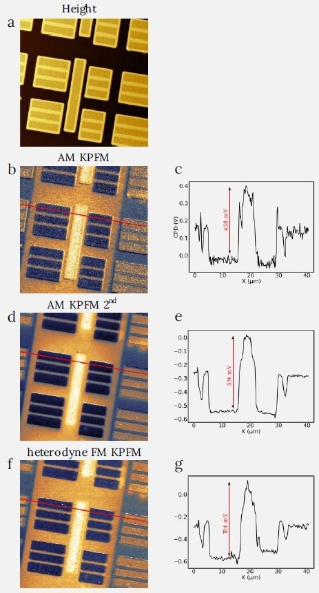
Figure 5. Comparison between the AM and FM KPFM modes on SRAM sample. The cross sections of the CPD scan demonstrate steady increase of difference between the maxium and minimum in CPD starting from the off-resonance AM KPFM, followed by the AM KPFM on 2^nd eigenmode and heterodyne FM KPFM. Image size: 40 x 40 μm². (a) height range: 600 nm, (b) CPD range: 0.55 V,  (c) CPD range: 0.61 V, (d) CPD range: 0.72 V.  (c), (e), (g) demonstate cross sections of (b), (d), (f), made along red lines. Image Credit: Nanosurf AG

The third sample measured is the semi-fluorinated alkane (F(CF₂)₁₄(CH₂)₂₀H or F14H20) sample. The semi-fluorinated alkanes is comprised of two parts – the soft hydrocarbon part, and the firmer fluorinated part.

The softer part typically attaches to the surface and these molecules create different self-organized structures on the substrate.⁹ Semi-fluorinated alkanes generally show good KPFM contrast and are often used as a standard sample to show the spatial resolution of the technique.

Figure 6 demonstrates how such a sample can be imaged with the same three modes, and it is clear to see, that the FM KPFM possesses the best lateral resolution of all three techniques. This corroborates the theoretical work regarding the size of the interaction volume in the FM KPFM mode.

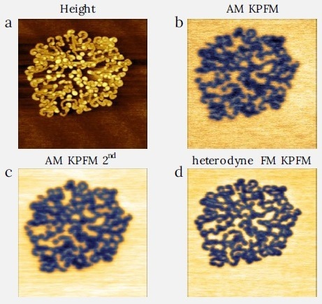
Figure 6. Comparison between the AM and FM KPFM modes on fluorinated alkane sample F14H20. Image size: 2 x 2 μm². FM KPFM shows best contrast.  (a) height range: 4 nm, (b) CPD range: 0.9 V, (c) CPD range: 1.1 V, (d) CPD range: 2 V. Image Credit: Nanosurf AG

Surface Charge and 2D Materials

While the phenomenological explanation of the Kelvin probe outlines the measurement of work functions, the KPFM technique is reactive to any electrostatic interaction and surface potentials. Resultingly, it is possible to image the distribution of surface charges that may appear after applying a local gate voltage.¹⁰

Another area of application is the study of charge-polarized superlattices produced by layers of twisted hexagonal boron nitride (hBN).¹¹ Figure 7 displays a sample in which an AM KPFM was used to capture an image at 2^nd resonance and with the heterodyne FM KPFM.

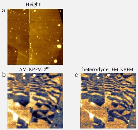
Figure 7. KPFM measurements of charge-polarized superlattices in twisted hexagonal boron nitride made with AM and FM KPFM. The FM KPFM is showing sharper image with finer details than the AM KPFM. Image size: 5.8 x 5.8 μm², (a) height range: 6.8 nm, (b) CPD range: 260 mV, (c) CPD range: 340 mV. Image Credit: Nanosurf AG

The charge superlattice is observed using both modes, and the image is a little sharper with the FM mode. 2D materials can also be imaged using KPFM, while extracting the information regarding their surface potential, which is of considerable importance for materials with thicknesses as small as one atom.

KPFM images of CVD graphene are exhibited in Figure 8, and here, as a result of the relatively large scan size, and smaller KPFM signal, the image quality is much improved with the application of AM KPFM at 2^nd resonance.

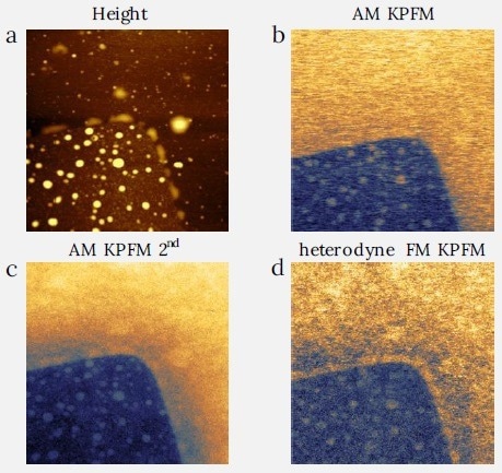
Figure 8. Comparison between the AM and FM KPFM modes on CVD graphene sample. Image size: 4.5 x 4.5 μm². (a) height range: 20 nm, (b) CPD range: 325 mV, (c) CPD range: 470 mV, (d) CPD range: 540 mV. Image Credit: Nanosurf AG

Calibration of the Tip Potential

Since KPFM is measuring the CPD voltage, which has been established as the difference of the potentials, for determining an accurate work function of the sample, the work function of the tip should also be known. In previous years, researchers have developed a variety of calibration procedures, including measuring the VCPD on highly oriented pyrolytic graphite (HOPG).

HOPG has been studied extensively and is often the preferred calibration sample due to its low cost, flatness, and ease of manipulation. The values reported for the work function are somewhere in the range of 4.5-5 eV. The dispersion of the work function is primarily related to surface contamination or inhomogeneities.¹²

Alternatively, it is possible to calibrate the probe by measuring the VCPD of a gold film, one previously characterized with ultraviolet photoelectron spectroscopy.^12,13 Gold is chosen due to its stability in the air, non-oxidizing properties, and being less vulnerable to the formation of a monolayer of water under ambient conditions.¹³

It should be noted that KPFM measurements calibrated under ambient conditions typically suffer from water, oxidation, and absorption of other contaminants on the surface. While the measurements in ultra-high vacuum conditions are comparatively expensive and labor-intensive, a compromise could be using a medium such as a nitrogen or argon-filled glovebox as an acceptable and cost-effective solution.

Conclusion

Modern KPFM is an essential and powerful electrical mode of AFM that measures surface potential. This is crucial across several domains of material research.

The heterodyne FM KPFM is a comparatively new KPFM mode, delivering the most appropriate measurement of the CPD voltage and, together with that, superior spatial resolution amongst other KPFM modes. The research community conclusively supports this.¹⁴

With the choice of shorter and softer cantilevers, it is possible to access better sensitivity to the surface potentials. It is necessary to control the calibration of the tip potential and ambient conditions to achieve the absolute measurement of the CPD.

References and Further Reading

1. Melitz, W., et al., Surface Science Reports 66 (2011) 1-27
2. Kelvin, Lord (1898). "V. Contact electricity of metals". The London, Edinburgh, and Dublin Philosophical Magazine and Journal of Science 46 (278) (1898) 82–120
3. Zisman, W. A., Rev. Sci. Inst. 3 (7) (1932) 367–370
4. J.M.R. Weaver and D.W. Abraham, J. Vac. Sci. Technol. B 9 (3) (1991) 1559-61
5. M. Nonnenma her, M.P. O’Bo le, and H.K. Wickramasinghe, Appl. Phys. Lett. 58 (1991) 2921-23
6. R. Borgani et al., Appl. Phys. Lett. 105 (2014) 143113
7. S. Magonov and J. Alexander, Beilstein J. Nanotechnol. 2 (2011) 15–27
8. T. Wagner et al., Beilstein J. Nanotechnol. 6 (2015) 2193–2206
9. A. Mourran et al., Langmuir 21 (2005) 2308-2316
10. S. Ye et al., Nanotechnology 32 (2021) 325206
11. C. Woods et al., Nature Communications (2021) 347
12. E. Castanon et al., J. Phys. Commun. 4 (2020) 095025
13. V. Panchal et al., Scientific Reports 3 (2013) 2597
14. A Axt et al., Beilstein J. Nanotechnol. 9 (2018) 1809–1819

This information has been sourced, reviewed and adapted from materials provided by Nanosurf AG.

For more information on this source, please visit Nanosurf AG.