In the realm of nanomechanical techniques, AFM is ideally suited to measuring soft materials because of its sub-nanometer vertical displacement accuracy and piconewton force resolution.
One of the most widespread mechanical measurements based on AFM is through force curves, also called force spectroscopy. To carry out these single point measurements, the cantilever moves towards and retracts from the surface, contacting the surface up to a pre-determined force.
The cantilever deflection is calculated as a function of z-actuator movement. These force curves provide an abundance of information that can be modeled through different contact mechanics models to obtain helpful characteristics like adhesion, elastic modulus, and stiffness. Force spectroscopy can be performed in either liquid or air environments.
Maps of force curves are also possible along with single-point measurement at specialized regions of interest. This allows localized mechanical property information to be correlated with topographical or other data acquired through the different imaging techniques.
How Does it Work?
Figure 1 provides an example of a sample’s force curves with z-actuator (piezo) movement on the x-axis and cantilever deflection on the y-axis. The force curve displays both the tip retracting from the sample in grey and approaching the sample in black.
For visibility, the grey withdrawing curve is drawn slightly under the black approaching curve, which prevents the curves from overlapping. The first observation is that the approach and retraction are hysteretic and do not align with each other everywhere.
In other words, the motion of the tip approaching the sample is not equivalent to the tip’s retraction motion, which reveals more information about the properties of the sample. The separate regions of the force curve are outlined below.
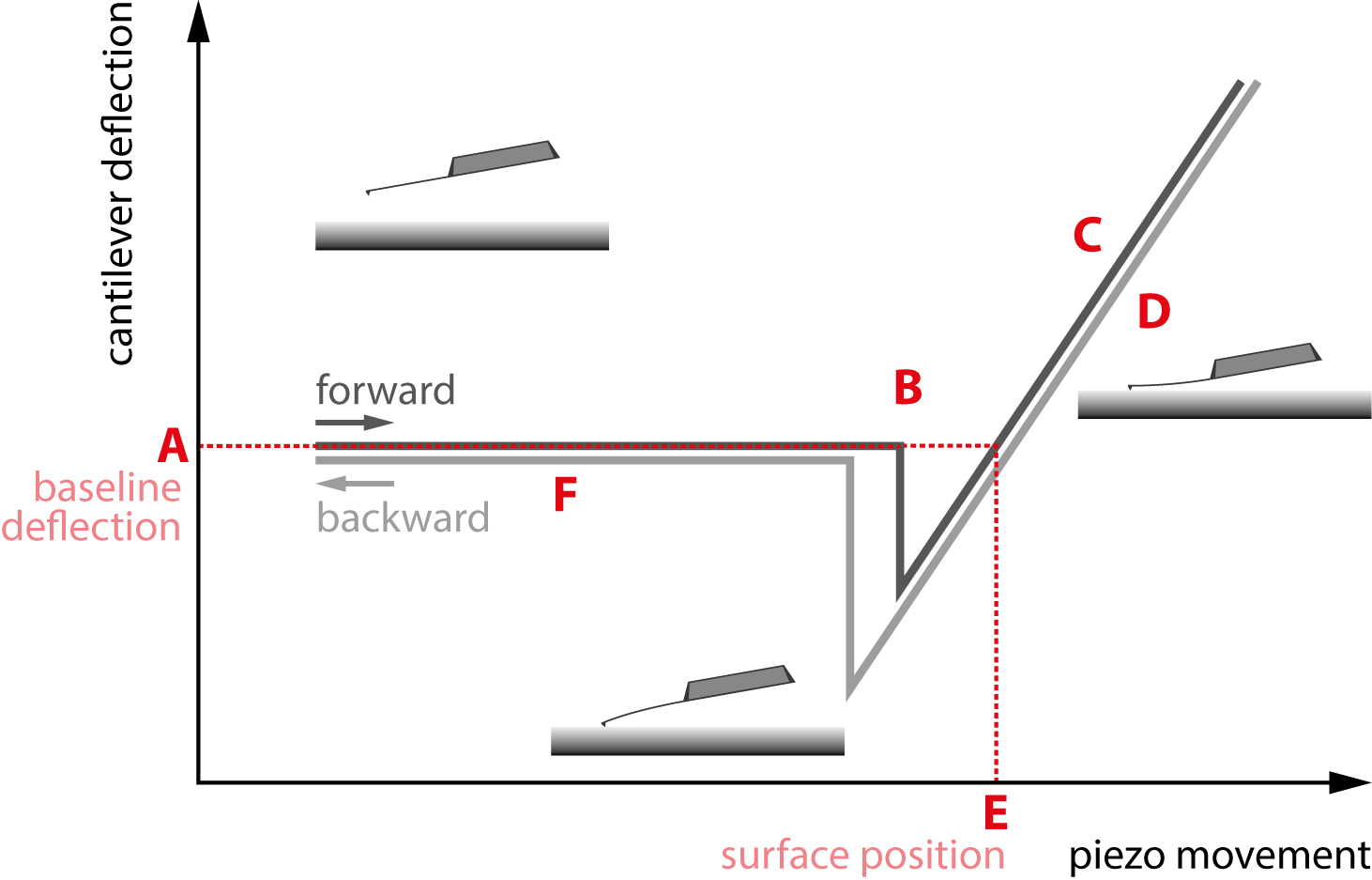
Figure 1. A standard force curve. The different regions of interest are marked A through F. Image Credit: Nanosurf AG
In the section labeled ‘A’, the tip approach starts with the cantilever above the surface. In the section labeled ‘B’, it launches into contact with the surface because of tip-sample interactions such as capillary forces.
The sloped section labeled ‘C’ is where the tip is in contact with the sample and begins to push against it. The cantilever will push into the sample until a force or deflection setpoint specified by the user is attained.
In section ‘D’, the tip begins to retract from the sample but can ‘stick’ to the surface as it withdraws. Due to this, a significant adhesive dip happens before the tip can finally impart from the surface and completely retracts, as displayed in section ‘F’.
It is important to note that when utilizing force curves to measure a property like elastic modulus, it is essential to carefully calibrate both the cantilever and the tip. The tip shape is one of the most critical calibrations.
For spherical tips, this is the radius, and for pyramidal or conical tips, this is the tip’s opening angle. Optical methods can be reliably employed to calculate the radius of the tip for spherical tips with a radius of several micrometers.
When calibrating tip shape for conical or pyramidal tips with a small radius, available techniques are reverse imaging of the tip by imaging a surface with features that are sharper than the tip, or direct imaging using a high-resolution technique like transmission or scanning electron microscopy.
Each of these techniques are inconvenient and still lack accuracy as neither account for variations in the geometry of the tip over time. As such, many users prefer to rely on the manufacturer’s specifications.
It is important to note that these specifications can be very unreliable, which then produces inaccuracy in the subsequent elastic modulus. This is the most significant source of error in this measurement.
The other calibrations that are necessary are related to the detector and cantilever. A technique called the ‘thermal method’ is most commonly used to calibrate the cantilever spring constant, which is where a power spectrum of a thermal cantilever tune (opposed to a piezo actuated tune) is obtained.
The obtained curve can be modeled with the equipartition theorem as a method to acquire the spring constant. Another widespread technique to calibrate the spring constant from the thermal cantilever tune is called the Sader method.
This technique is based on a model describing how the hydrodynamics of the surrounding medium influences the motion of the cantilever while accounting for the geometry of the cantilever.
Determining the optical lever’s deflection sensitivity is the final calibration stage. Volts calculated on the photodetector are converted to nanometers of cantilever deflection in this stage.
This is achieved by conducting a force curve on an incompressible sample such as sapphire, glass, or silicon. The sample must be hard enough to ensure that its compression is insignificant compared to the cantilever’s deflection at the applied force. The photodetector’s changes in voltage will be relative to the deflection of the cantilever when the compression of a sample is negligible.
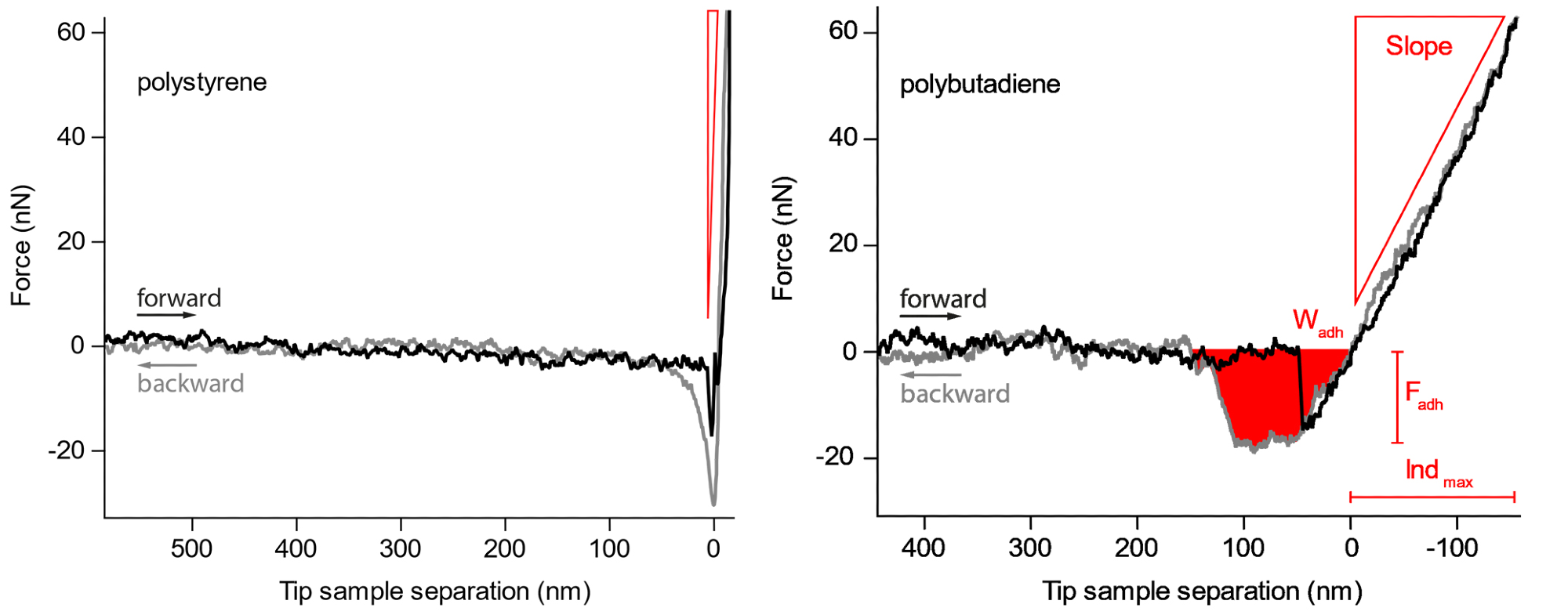
Figure 2. Force curves on the harder polystyrene and the softer polybutadiene. The slope, maximum adhesion force, and work needed to retract the cantilever from the sample are readily observed. Image Credit: Nanosurf AG
Figure 2 provides an example where individual curves have been acquired on a blend of polybutadiene (bottom) and polystyrene (top).
As both of these polymers significantly differ in regards to adhesion and elastic modulus, they provide an effective example of how force curves can correctly distinguish these properties in different materials.
The black curve follows the tip as it withdraws from the surface while the grey curve depicts the motion of the tip as it approaches the surface. Region ‘C’ displays a key difference in the slope of the repulsive wall of the force curve where the polystyrene material clearly demonstrates a slope that is much steeper than the polybutadiene. This suggests that polystyrene has a higher elastic modulus compared to polybutadiene.
The adhesion section of the curve also varies significantly. The polystyrene has a larger adhesive dip (down to approximately 30 nN) suggesting larger adhesion, while the region of the adhesive dip in the polybutadiene is more significant, suggesting a larger work of adhesion.
The force curve data must be modeled with a contact mechanics model after collection to obtain the stiffness or elastic modulus data. JKR, DMT, Sneddon, and Hertz are the four key models used for AFM tip-sample interactions.
The Sneddon and Hertz models do not account for any adhesion between the sample and tip, which makes them suitable for samples that do not stick in relation to the tip.
While the Hertz model assumes an indentation smaller than the tip radius and a spherical tip shape, the Sneddon model is a more general technique, including a broader range of tip shapes like pyramidal and conical, which are frequently more suitable when describing the tip of a regular AFM cantilever.
The majority of samples do display a type of adhesion on the nanoscale and a model that takes this into consideration is usually necessary, but the approach curves can still be described in a general manner by the Sneddon and Hertz models.
Long-range attractive forces are added to the Hertz area to include adhesion beyond the contact area in the DMT model. The slope of the repulsive wall (area D) is suitable to obtain the elastic modulus in the DMT model.
The JKR model considers the stronger adhesion that happens inside of the contact area. This model additionally considers the hysteresis when the tip withdraws from or approaches the sample.
The 2-point JKR model, a modified version of the JKR model, is frequently employed to obtain the elastic modulus and it models the adhesive region of the curve (region E).
Applications
A ‘force map’ can be created which is where individual force curves are collected in an array on the sample and a force curve is obtained at each pixel. Mechanical characteristics can be determined from each of these curves to construct corresponding property maps, for example elastic modulus or adhesion.
In this example, a force map was gathered on epithelial cells. The maximum adhesion force was determined from individual force curves and the curves were fitted for the elastic modulus information.
Figure 3 depicts the adhesion map, where the adhesion data was “painted” onto the 3D topography to enhance the visual representation of this sample. The fitted contact point of each force curve was used to determine the sample weight and to produce a zero-force sample topography.
Across the surface of the cell, a homogeneous adhesion value is noted. The histogram also measures the adhesion, which suggests that most adhesion occurring in the cell has a force of around 0.15 to 0.20 nN.
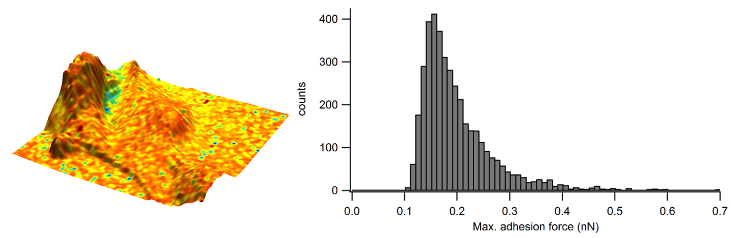
Figure 3. Adhesion overlaid in color on the 3D representation of the sample height and corresponding adhesion distribution as a histogram. Image Credit: Nanosurf AG
Figure 4 displays a map of the elastic modulus. In this example, the elastic modulus has been mapped onto the 3D topography and demonstrates that elastic modulus is diverse across the surface of the cell.
The bright purple regions represent high elastic modulus values whereas the red regions represent low elastic modulus values. The histogram also measures these values and shows that the taller regions of the cells have an elastic modulus less than 5 kPa, surrounded by a surface with an elastic modulus reaching between 10 to 15 kPa.
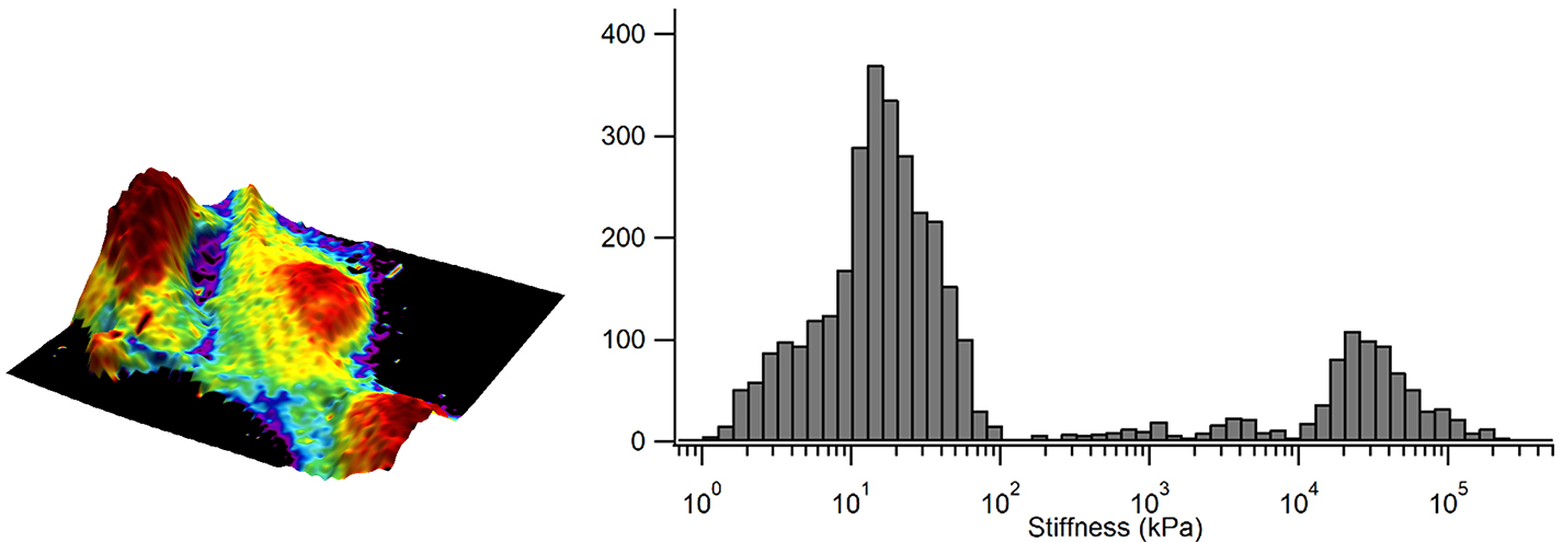
Figure 4. Elastic modulus overlaid in color on the 3D representation of the sample height and corresponding elastic modulus distribution as a histogram. Image Credit: Nanosurf AG
Measuring the properties of hydrogels is another application of force spectroscopy. Hydrogels are an important category of materials with applications in the consumable and medical industries.
Hydrogels have a variety of uses and consist of a network of polymer chains with a high content of water. As these materials must be hydrated and are very soft, on the order of a few kPa, they are difficult to analyze with any technique other than AFM.
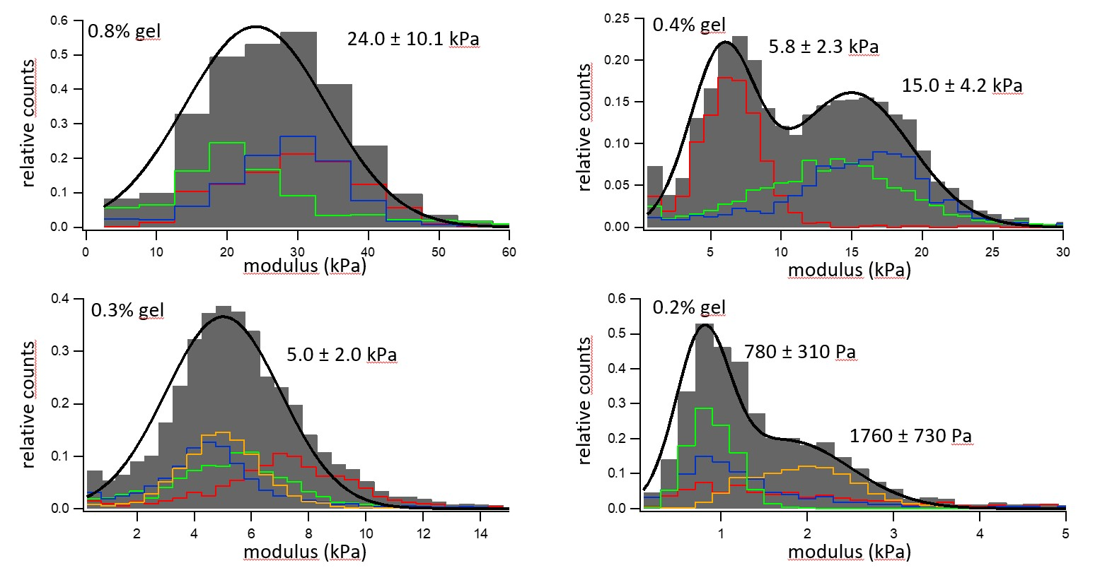
Figure 5. Elastic modulus distribution of four hydrogels with different concentrations of gelatin. Image Credit: Nanosurf AG
Figure 5 displays the data from four individual hydrogel materials with different concentrations of gelatin, which were quantified with force curves in situ under an aqueous solution.
Histograms of the moduli are depicted where the colored histograms constitute separate 30 µm x 30 µm sample regions. The grey bins represent an aggregated histogram of each separate area, which has been fitted to a double or single Gaussian distribution in the black line.
The first trend which can be seen is that materials which have a larger hydrogel component are stiffer. This varied from a material which was 0.8% gel with an elastic modulus of 24 kPa to a material which was 0.2% gel and had an elastic modulus of around 1 kPa.
Additionally, the materials exhibit a significant difference in elastic modulus from various probed regions, indicating a spatial heterogeneity in the sample’s gel composition. This highlights the requirement to repeat these measurements on a large spatial scale.
Summary
AFM is ideally designed to quantify nanoscale mechanical properties due to its sub-nanometer displacement resolution and its piconewton force, particularly in the case of soft materials.
Force spectroscopy is a helpful nanomechanical method to acquire maps of key mechanical properties like stiffness (elastic modulus) and adhesion, along with single-point measurements.
Tip and cantilever calibrations along with contact mechanics models provide the complete interpretation and analysis of distinct force curves. Applying force curves to a wide range of materials has been outlined in this article including the measurement of hydrogels, polymers, and cells.

This information has been sourced, reviewed and adapted from materials provided by Nanosurf AG.
For more information on this source, please visit Nanosurf AG.