AFM is particularly well-suited to working with soft materials in the field of nanomechanical measurements, owing to its piconewton force resolution and sub-nanometer vertical displacement accuracy.
One of the most common AFM-based mechanical measurements is conducted via force curves, otherwise referred to as force spectroscopy. To conduct such single point measurements, the cantilever moves towards and retracts away from the surface, touching the surface up to a pre-defined force.
The z-actuator movement can be used to determine the cantilever deflection. These force curves are comprised of a plethora of information that a number of contact mechanics models can model to pull out valuable properties such as adhesion, elastic modulus, and stiffness.
Force spectroscopy can be performed in both liquid and air environments. In addition to single point measurement at localized regions of interest, maps of force curves are also viable. This facilitates the association of localized mechanical property information with topographical or other information acquired by the different imaging methods.
How does it work?
In Figure 1, a sample force curve is displayed with cantilever deflection on the y-axis and z-actuator (piezo) movement on the x-axis. The force curve depicts both the approach of the tip towards the sample in black and the withdrawal of the tip from the sample in grey.
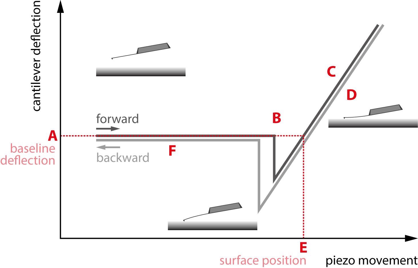
Figure 1. A standard force curve. The different regions of interest are marked A through F. Image Credit: Nanosurf AG
By way of illustration, the grey withdrawing curve is drawn just beneath the black approach curve, hence avoiding any overlap of the curves. The initial observation is that the approach and withdrawal do not follow each other throughout; they are hysteretic.
That is to say, the tip’s motion towards the sample is not the same as the tip withdrawal motion, a fact that offers further information about the sample properties. The particular regions of the force curve are detailed below.
The approach of the tip begins with the cantilever above the surface in the region marked “A.” It then clicks into contact with the surface in the region marked “B” as a result of tip-sample interactions like capillary forces.
At this point, the tip and sample are in contact, and the tip pushes against the sample in the sloped region marked “C.” The cantilever will push into the sample until a deflection or force setpoint set by the user is reached.
The tip withdrawal then starts in region “D” but may “stick” to the sample surface as it is pulled out. Resultingly, a large adhesive dip appears before the tip is finally able to escape the surface and completely withdraw, as displayed in section marked “F.”
One critical factor to note when utilizing force curves to measure a property such as elastic modulus is the necessity to carefully calibrate both the tip and cantilever. One of the most crucial calibrations is that of the tip shape.
This is the opening angle of the tip in relation to conical or pyramidal tips, and for spherical tips, it is the radius. For spherical tips with radii of several micrometers, optical techniques can be used to accurately measure the tip radius.
Some of the techniques of tip shape calibration that are available for small radius tips with pyramidal or conical tips include high-resolution direct imaging techniques like scanning or transmission electron microscopy or by imaging a surface with features that are sharper than the tip using reverse imaging.
Both are awkward and flawed as none of these methods take changes in tip geometry over time into consideration. Hence, most users prefer to trust manufacturer specifications.
It is crucial to recognize that there can be considerable uncertainty in these specifications that then leads to uncertainty in the resulting elastic modulus; it is the greatest source of error in this measurement.
Other necessary calibrations are typically associated with the cantilever and detector. The cantilever spring constant is usually calibrated using the “thermal method,” in which a power spectrum of a thermal cantilever tune (instead of a piezo actuated tune) is acquired.
One possible way to acquire the spring constant is to model the relative curve with the equipartition theorem. Another frequently used method is to calibrate the spring constant from the thermal cantilever tune. This is referred to as the Sader method.
The Sader method is reliant on a model that is predicated on the influence of the hydrodynamics of the surrounding medium on the cantilever motion while at the same time taking the geometry of the cantilever into consideration.
The last stage of calibration is determining the deflection sensitivity of the optical lever. This facilitates the conversion of volts measured on the photodetector to nanometers of cantilever deflection.
It is achieved by applying a force curve on an impenetrable sample like silicon, sapphire or glass. The sample has to be hard enough that its compression is negligible in comparison with the deflection of the cantilever at the applied force.
When there is negligible compression of the sample, the changes in voltage from the photodetector will match the deflection of the cantilever. For instance, individual curves taken from a blend of polystyrene (top) and polybutadiene (bottom) are displayed in Figure 2.
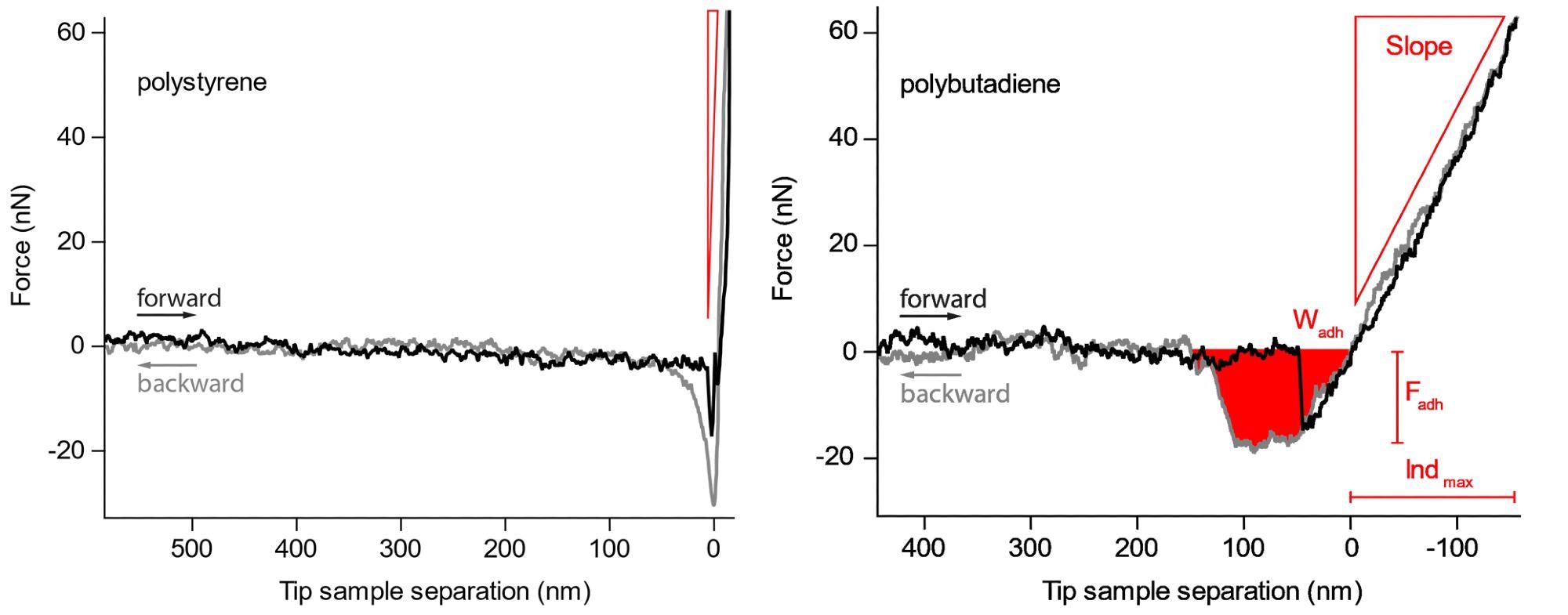
Figure 2. Force curves on the harder polystyrene and the softer polybutadiene. The slope, maximum adhesion force and work needed to retract the cantilever from the sample are readily observed. Image Credit: Nanosurf AG
These two polymers greatly differ in their elastic modulus and adhesion and therefore offer the perfect illustration of how force curves can effectively differentiate these properties on various materials.
The grey curve is the motion of the tip’s approach towards the surface, while the black curve traces the tip as it withdraws from the surface.
One significant difference is the slope of the repulsive wall of the force curve (area “C”), where the polystyrene material clearly indicates a far steeper slope compared to that of the polybutadiene, stressing that the polystyrene has a higher elastic modulus than polybutadiene.
Moreover, the adhesion part of the curve is also extremely different where the polystyrene has a grater adhesive dip (down to approx. -30 nN), signifying larger adhesion. In contrast, the area of the adhesive dip in the polybutadiene is greater, demonstrating a larger work of adhesion.
Once force curve data acquisition is complete, it must be modeled with a contact mechanics model to obtain the information related to elastic modulus or stiffness.
There are four primary models used for AFM tip-sample interactions: Sneddon, Hertz, JKR and DMT. The Hertz and Sneddon models are unable to determine any adhesion between the tip and sample, making them best suited for “non-sticky” samples with respect to the tip.
While the Hertz model assumes the tip is a spherical shape and the indentation is smaller than the tip radius, the Sneddon model is a broader approach, including a greater variety of tip shapes that include conical and pyramidal. Such shapes are usually better suited when describing the tip of a standard AFM cantilever.
The majority of samples do demonstrate some form of adhesion on the nanoscale, and thus a model that takes this into account is typically required, although the approach curves can usually still be described by the Hertz and Sneddon models.
The DMT model introduces long range attractive forces to the Hertz area to account for adhesion outside the contact area. In the DMT model, the slope of the repulsive wall (region D) is suitable for the extraction of the elastic modulus.
The JKR model offers an explanation for stronger adhesion that occurs within the contact area; this model also considers the hysteresis in the approach and withdrawal of the tip from the sample. A refined version of the JKR model, called the 2-point JKR model, is typically used to extract the elastic modulus, and it models the curve’s adhesive portion (region E).
Applications
Individual force curves can be amassed in an array on the sample, generating a “force map” where a force curve is collected at each pixel, and mechanical properties can then be retrieved from each force curve to produce equivalent maps of properties such as adhesion or elastic modulus.
A force map was generated for epithelial cells. From individual force curves, extraction of the maximum adhesion force was conducted, and curves were adapted for the elastic modulus data. The adhesion map is displayed in Figure 3, where the adhesion was “painted” onto the 3-D topography to maximize the visualization of this sample.
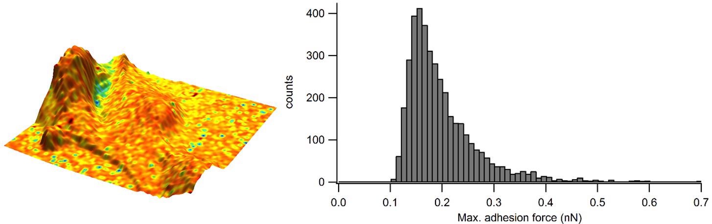
Figure 3. Adhesion overlaid in color on the 3D representation of the sample height and corresponding adhesion distribution as a histogram. Image Credit: Nanosurf AG
In order to acquire a so-called zero-force sample topography, the sample height was calculated from the fitted contact point of each force curve. A rather homogenous value of adhesion is established across the cell surface. The adhesion is quantified further using the histogram, which indicates that frequently occurring adhesion has a force of approximately 0.15-0.20 nN.
A map of the elastic modulus is displayed in Figure 4, where this time, the elastic modulus has been “painted onto” the 3-D topography and demonstrates a heterogeneous elastic modulus across the surface of the cell.
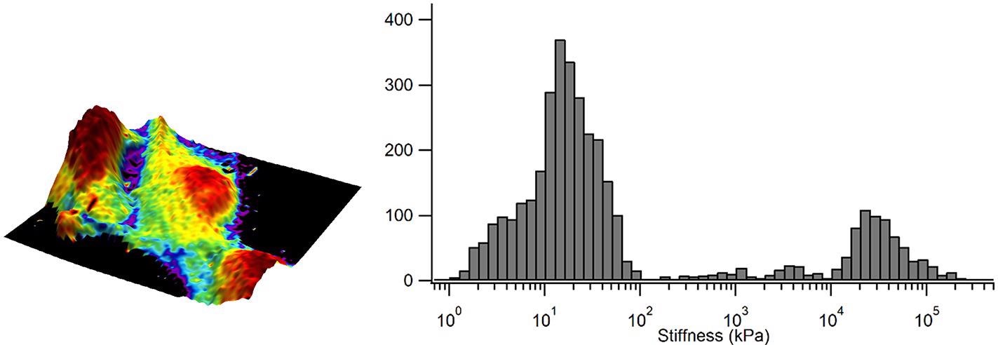
Figure 4. Elastic modulus overlaid in color on the 3D representation of the sample height and corresponding elastic modulus distribution as a histogram. Image Credit: Nanosurf AG
The red areas signify low elastic modulus values and bright purple are indicative of high elastic modulus values. The histogram further quantifies these values and shows that the elastic modulus of the taller areas of the cells is below 5 kPa surrounded by a surface with an elastic modulus that peaks between 10-15 kPa.
An additional example of force spectroscopy usage is to measure the properties of hydrogels, an essential class of materials with applications in the medical and consumable industry. Hydrogels are made up of a network of polymer chains with a high content of water and have a variety of uses.
Due to the softness of these materials – on the order of few kPa – and the fact they must be hydrated, it is a challenge to measure them with any method other than AFM.
The data taken shown in Figure 5 relates to four different hydrogel materials with different gelatin concentrations that have been measured with force curves in situ under an aqueous solution.
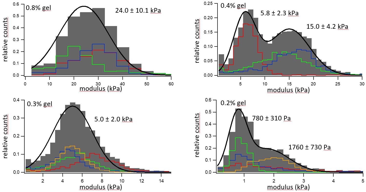
Figure 5. Elastic modulus distribution of four hydrogels with different concentrations of gelatine. Image Credit: Nanosurf AG
Histograms of the moduli are displayed where the colored histograms are indicative of different 30 µm x 30 µm areas on the sample, and the grey bins portray an aggregated histogram of all the single regions, which has been aligned with a single or double Gaussian distribution in the black line.
The first trend seen is that materials with the greater hydrogel component are stiffer, ranging from a material that was 0.8% gel with an elastic modulus of 24 kPa to a material that was 0.2% gel and had an elastic modulus of around 1 kPa.
Secondly, the materials demonstrate a greater variation in elastic modulus from various areas probed, reflecting a spatial heterogeneity in gel composition in the sample, highlighting the need to repeat these measurements on a larger spatial scale.
Summary
Exploiting its piconewton force and sub-nanometer displacement resolution, AFM is extremely well-suited to measure nanoscale mechanical properties, particularly when it comes to soft materials.
Force spectroscopy is a practical nanomechanical technique to acquire both single point measurements and maps of key mechanical properties, including adhesion and stiffness (elastic modulus).
Cantilever and tip calibrations paired with contact mechanics models facilitate the complete analysis and interpretation of individual force curves. The application of force curves to a broad range of materials is shown in this article, including measurements of polymers, cells and hydrogels.

This information has been sourced, reviewed and adapted from materials provided by Nanosurf AG.
For more information on this source, please visit Nanosurf AG.