Abstract
Three samples of shale rock, two from the Eagle Ford play and one from the Haynesville play, were successfully tested by instrumented indentation using a Nano Indenter G200 from KLA.
Results were remarkably repeatable, and hardness and Young’s modulus were independent of force for test forces above 300mN. For the two samples from the Eagle Ford play, the reduced moduli were 54.3GPa and 40.6GPa, and the hardness values were 1.55GPa and 1.12GPa. For the Haynesville sample, the modulus was 22.5GPa and the hardness was 0.51GPa. By assuming a Poisson’s ratio of 0.25 and negligible work-hardening, stress-strain curves were deduced from these indentation measurements.
Finite-element simulations of indentation experiments were conducted wherein the simulated materials were assigned the deduced stress-strain curves. Simulated force-displacement curves matched experimental force-displacement curves reasonably well, thus lending credibility to the material model and to the indentation method of determining constitutive properties.
Introduction
Shale formations host vast natural gas and oil reserves that are accessed by hydraulic fracturing. Experts in the oil and gas industry have analytical tools at their disposal for optimizing fractures to maximize the productivity of a well, and these analytical tools require knowing the stress-strain curve for the shale, as well as other mechanical properties.
The simplest elastic-plastic constitutive model is illustrated schematically in Figure 1 as a bilinear stress-strain curve. Materials for which this model is appropriate experience elastic deformation so long as the principal stress remains below the yield stress, Y. The primary characterization of the elasticity of the material is the Young’s modulus, E, which is the slope of the stress-strain curve prior to the onset of plasticity.
For isotropic materials, elasticity is fully described by the Young’s modulus and the Poisson’s ratio, v. For stresses above the yield stress, the material deforms plastically, exhibiting large strains for relatively small increases in stress. If the material has a capacity for work-hardening, then the stress-strain curve has a positive slope, F, beyond the yield point.
If the material has no capacity for work-hardening, then the stress-strain curve is flat beyond the yield point (F = 0). In summary, such materials are mechanically described by only four parameters: Young’s modulus (E), Poisson’s ratio (ν), yield stress (Y), and hardening slope (F).
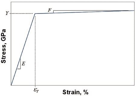
Figure 1. Idealized bilinear stress-strain curve that requires four material constants for full definition: E, ν, Y, F.
Indeed, shale is a complex composite of clay, minerals, and organic material. Yet there are reasons to hope that at large scales, relative to the microstructure, shale might succumb to a simple mechanical model like that illustrated in Figure 1, and that further, instrumented indentation might be used to obtain essential mechanical properties.
Thus, an obvious question arises: If instrumented indentation is used to measure the mechanical properties, how large must the indentations be in order to measure properties that are relevant and representative of the bulk material?
In the present work, we develop a methodology by which this question may be answered generally, and we apply that methodology to three specific shale samples. Finally, we verify both the constitutive model and the properties obtained via indentation using finite-element analysis by comparing experimental and simulated force-displacement data.
From this comparison between simulation and experiment, we speculate about how the constitutive model might be improved to more closely represent the true mechanical behavior of the shale.
Review of Instrumented Indentation Theory
For two smooth, isotropic, axisymmetric bodies in elastic contact, the reduced elastic modulus (Er), contact stiffness (S), and contact area (A) are related as.
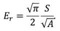 (1)
(1)
The reduced elastic modulus incorporates bi-directional displacements in both contacting bodies, and is related to the Young’s modulus, E, and Poisson’s ratio, ν, of each body as
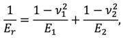 (2)
(2)
where the numerical subscripts identify each of the two contacting bodies.
In instrumented indentation, these idealized relations are presumed to govern the contact between the indenter and the test material. Even when the indentation causes significant plasticity, these expressions remain relevant because the two bodies, even once deformed by plasticity, retain the ability to interact elastically according to Eq. 1.
Thus, the purpose of an instrumented indentation test is to cause a controlled contact during which measurements are made to determine the contact stiffness, S, and contact area, A, so that reduced modulus, and ultimately, the Young’s modulus of the test material can be determined.
During a basic instrumented indentation test, contact force, P, and penetration, h, are continuously recorded for the entire time that the indenter is in contact with the material.
Additional information about the contact can be achieved by superimposing a small oscillation on the indenter and monitoring the amplitude ratio, Fo/zo, as well as the phase shift, φ. Contact stiffness, S, can either be calculated as the slope of the force-penetration data acquired during unloading, which manifests elastic recovery, or as the real part of the amplitude ratio of the superimposed oscillation.
The contact area is deduced in two steps. First, the contact depth, hc, is calculated by subtracting the normal surface deflection, hs, from the total measured penetration:
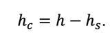 (3)
(3)
The same elastic contact analysis by which Eq. 1 is derived also gives us an expression for hs, which is
 (4)
(4)
Second, the contact area, A, is calculated from the contact depth, hc, using an “area function” that describes the known geometry of the indenter:
 (5)
(5)
By these means, contact stiffness, S, and contact area, A, are determined by instrumented indentation, thus allowing the calculation of reduced modulus, Er, by Eq. 1. If the Poisson’s ratio of the test material, ν, is known a priori, then the Young’s modulus of the test material can be calculated from Eq. 2 as:
 (6)
(6)
Where Ei and νi are the Young’s modulus and Poisson’s ratio of the diamond, which are 1140GPa, and 0.07, respectively.
In an instrumented indentation test, the hardness, H, is defined simply as
 (7)
(7)
For many materials, the hardness is simply proportional to the yield stress of the material, Y, with the constant of proportionality being about 3:
 (8)
(8)
Although in theory it is possible to determine the post-yield hardening behavior of a material by means of an instrumented indentation test, this cannot be done with the common Berkovich indenter. Because the Berkovich indenter is a self-similar pyramid, it gives rise to a strain field that grows only in extent with increasing force, not in shape or magnitude.
For this reason, the Berkovich indenter is said to cause a single effective strain, not because the strain everywhere is the same, but because the strain field does not change with force, except to grow in extent, proportionally to the size of the indentation. (By contrast, a spherical indenter gives rise to a strain field that does change in both shape and magnitude, as well as extent, as the applied force increases.
The strain field gradually becomes more severe, with more plastic deformation, as the indenter is pushed further into the material. Thus, spherical indenters are usually employed for characterizing the post-yield hardening of a material by indentation.)
For materials that manifest creep, the yield stress depends on strain rate. For such materials, the hardness also depends on strain rate due to the proportional relationship between hardness and yield stress.
If the indentation strain rate is higher (i.e., faster), it gives rise to a higher flow stress, which in turn gives rise to a proportionally higher hardness. In an indentation test, the strain rate is best defined as the loading rate divided by the load (P./P).
Even when the goal of testing is not to characterize creep per se, one should appreciate that the indentation strain rate must be controlled in order to arrive at a meaningful value of hardness. The Dorn constitutive model for creep, rendered for indentation is
 (9)
(9)
Where B and m are constants that depend on temperature and microstructure, and ε. is the indentation strain rate. Thus, in materials that manifest creep, ε.= P./P must be maintained at a constant value throughout the indentation experiment in order to achieve a constant value of hardness. In other words, as the applied force, P, increases, so must the loading rate, P..
As a counter example, indentation standards typically prescribe testing with a constant loading rate. However, such a protocol is inappropriate for materials that creep, because if the loading rate, , P., is held constant, then the strain rate, P./P, will decrease as the indentation progresses, because the applied force, P, increases.
In materials that creep, a constant-loading-rate or constant-displacement-rate protocol gives rise to a hardness that continuously decreases with applied force or displacement. Thus, if the potential for creep is suspected, the best indentation protocol is to apply force in such a way as to hold P./P at a constant value.
Experimental Method
Three samples of shale were tested. The first two samples were from the Eagle Ford play, though not from the same geographic area. The third sample was from the Haynesville play. The size of each sample was about 4mm x 3mm x 1mm. The first sample from the Eagle Ford play was mechanically polished down to a 0.5 micron grit size. The second sample from the Eagle Ford play was given a smooth mechanical cut, then ion milled for a few hours on a dual-beam argon milling system. The sample from the Haynesville play was also ion milled after a first mechanical pass. Generally, the ion-milling process was preferred for sample preparation because it required less human practice and attention. Table 1 summarizes the samples and their preparation.
Table 1. Sample descriptions.
| ID |
Geographic source |
Sample Preparation |
| 1 |
Eagle Ford |
Mechanically polished down to a 0.5 micron grit size. |
| 2 |
Eagle Ford |
Fine mechanical cut, then ion-milled with dual-beam Ar laser. |
| 3 |
Haynesville |
Fine mechanical cut, then ion-milled with dual-beam Ar laser. |
All indentation testing was performed with a KLA Nano Indenter G200, configured with a KLA XP head, a Berkovich indenter, and the KLA continuous stiffness measurement (CSM) option. The CSM option allows the superposition of a small oscillation (2nm at 45Hz) so that the contact stiffness, S, can be determined as the real part of the amplitude ratio, S = (Fo/zo)cosφ.
The primary benefit of this technique is that properties can be measured continuously during loading while the strain rate is well controlled. The loading rate divided by the load, P./P, was controlled during loading to be 0.05/sec. When the maximum indentation force of 550mN was reached, the force was held constant for a dwell time of 10 seconds prior to unloading. With this test method, each indentation yielded channels of reduced modulus, Er, and hardness, H, calculated continuously during loading by Eqs. 1 and 7, respectively.
Eight indentation arrays were performed on each sample. Each array comprised nine indentations, within a domain of 200µm x 200µm (individual indents in the array were separated by 100µm in each direction). Thus, a total of 72 indentations were performed on each sample: 8 arrays x 9 indents per array = 72 indents. The eight arrays were arranged so as to span the available sample surface. One array was performed in each of the four corners, and four more arrays were performed near the center of the sample. After testing all three samples, shale #2 was tested a second time by exactly the same procedure.
Data from the 72 indentions on each sample were consolidated in the following manner. For each indentation, reduced modulus and hardness were calculated at five forces: 100mN, 200mN, 300mN, 400mN, and 500mN. Logistically, this was accomplished by averaging all data in the Er and H channels within ±10mN of the target force.
For example, for the first indent performed on shale #1, the reduced modulus at 100mN was calculated as the average of the measured values in the Er channel for which the applied force was between 90mN and 110mN. Then, from each array of nine indents, the median values of reduced modulus and hardness were retained for each force. In other words, each array yielded five median values of reduced modulus — one for each force, and five median values of hardness. (Taking the median values from each array naturally filtered outliers, thus eliminating human biasin data reduction.)
Finally, the reported properties for each force were calculated as the mean and standard deviation of the eight median values (one for each array) for that force. In effect, each array of nine indentations is considered to be a single test on the shale, and the medians are considered to be the primary results of that test.
In order to discover the minimum force for testing, the student’s t-test was used to discern whether the properties measured at different forces were significantly different. For example, on shale #1, the student’s t-test was used to compare the reduced modulus obtained at 100mN with that obtained at 500mN. In any pair-wise comparison between results at two different forces, the degree of freedom was 14 (8+8-2), as the means and standard deviations used in the student’s t-test were calculated across eight median values.
With the reduced modulus and hardness directly measured as described above, we were able to estimate the four parameters needed to describe each material with a bilinear stress-strain curve. The Young’s modulus was computed according to Eq. 7 assuming a Poisson’s ratio of ν = 0.25. (Sensitivity analysis of Eq. 7 reveals that if the true bulk Poisson’s ratio of the shale is in the range of 0.15–0.35, then the error in Young’s modulus associated with assuming ν = 0.25 is less than 5%.)
The yield stress was calculated by Eq. 8, with the constant of proportionality being exactly 3. Finally, no mechanism for work-hardening seemed obvious to us, so we presumed a very slight degree of hardening, set at 1% of the value of the Young’s modulus. (Indeed, we would have preferred to set F = 0, but this did not lend itself to numerical convergence of subsequent finite-element simulations.)
Finite-Element Simulations
We performed three axisymmetric finite-element simulations of indentation experiments using Cosmos 2.8. For the first simulation, the test material was assigned the constitutive properties (E, ν, Y, F) that were determined for shale #1; the second and third simulations were likewise performed with the test material having the constitutive properties determined for shale #2 and shale #3, respectively. The output of each simulation was a simulated force- displacement curve. The force-displacement curve from the first simulation was compared to an experimental force-displacement curve from shale #1 for an indentation that happened to have reduced modulus and hardness (at 500mN) that were within 2% of the values determined for the bulk material. The force- displacement curves from the second and third simulations were likewise compared to typical experimental force-displacement curves from shale #2 and shale #3, respectively.
The simulated indenter was a cone having an area function identical to that determined for the physical Berkovich indenter used for testing (A = 23.9305d2 + 1312.33d, where d was the distance from the apex along the axis of the indenter, expressed in nm.) The indenter was defined to be a linear-elastic material having the properties of diamond: Ei= 1140GPa and νi= 0.07.
Results and Discussion
Figure 2 shows the results for a single array of nine tests on shale #1, along with an optical image of the residual indentation. For each indentation, the reduced modulus and hardness are calculated as a semi-continuous function of indentation force. Such traces are extraordinarily useful and can only be achieved by oscillating the indenter as it proceeds into the material.
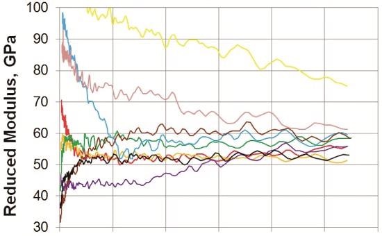
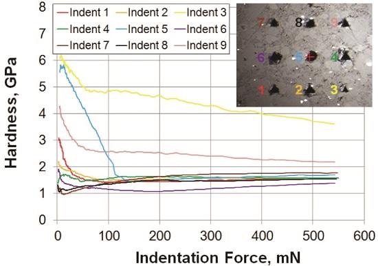
Figure 2. (a) Reduced modulus and (b) hardness as a function of indentation force for the first array of nine indents on shale #1. At intervals of 100mN, the median value of each property was taken as representative of the array.
In Figure 2, the optical image informs our interpretation of the quantitative measurements. From the optical image, we see that indent 3 left the smallest indentation at the peak force of 550 mN, and indeed, this test returned the highest measurement of both reduced modulus and hardness. The roundness of indent 5 indicates that it may have caused material to spall away, which comports with the sharp drop in reduced modulus and hardness within the first 100mN. Interestingly, we see a crack emanating from the corner of indent 9 that appears to be contained within a single particle. This crack may be the source of the drop in modulus at about 220mN. Indeed, something interesting may well be learned from each test by interpreting the quantitative data in view of the actual indentation.
Yet, we must make sense of the material as a whole. Taking median properties as representative of each array of nine indents is a good way to reduce the sensitivity of the final result to outlying measurements. For example, in Figure 2a, despite the apparent variation in modulus with test site and force, the medians are remarkably consistent. In order of increasing force, the median reduced moduli for this array (in GPa) were 57.5, 56.4, 57.1, 56.4, and 56.4. It should be noted that the median values do not necessarily come from the same test at each force. From Figure 2a, we see that at 100mN, it is indent 7 that provides the median reduced modulus (57.5), whereas at 500mN, it is indent 4 that provides the median (56.4).
Table 2 provides the mean and standard deviation for each collection of eight medians. For example, the first entry in Table 2 is the mean of the eight median values of reduced modulus obtained at 100mN, one median value coming from each array of nine indentations.
Table 2. Properties measured at five different indentation forces. Red outline indicates that result differs significantly from those measured at one or more higher forces (student’s t-test, 95% confidence).
| |
Reduced modulus (GPa) |
Hardness (GPa) |
| Material |
100 mN |
200 mN |
300 mN |
400 mN |
500 mN |
100 mN |
200 mN |
300 mN |
400 mN |
500 mN |
| |
Avg. |
Dev. |
Avg. |
Dev. |
Avg. |
Dev. |
Avg. |
Dev. |
Avg. |
Dev. |
Avg. |
Dev. |
Avg. |
Dev. |
Avg. |
Dev. |
Avg. |
Dev. |
Avg. |
Dev. |
| Shale 1 |
53.2 |
4.72 |
53.6 |
2.88 |
53.7 |
2.74 |
53.9 |
2.23 |
54.3 |
2.66 |
1.62 |
0.25 |
1.55 |
0.19 |
1.54 |
0.16 |
1.55 |
0.18 |
1.55 |
0.14 |
| Shale 2 |
42.3 |
3.06 |
41.5 |
1.67 |
41.0 |
1.78 |
41.5 |
1.48 |
40.6 |
1.83 |
1.26 |
0.20 |
1.19 |
0.13 |
1.14 |
0.10 |
1.13 |
0.10 |
1.12 |
0.09 |
| Shale 3 |
25.7 |
3.27 |
24.0 |
3.56 |
23.3 |
3.58 |
22.6 |
3.63 |
22.5 |
3.83 |
0.65 |
0.11 |
0.61 |
0.07 |
0.57 |
0.07 |
0.52 |
0.10 |
0.51 |
0.10 |
| Shale 2 (Rep) |
41.3 |
3.58 |
40.3 |
2.52 |
40.1 |
2.59 |
39.7 |
2.43 |
40.0 |
2.36 |
1.18 |
0.12 |
1.14 |
0.11 |
1.13 |
0.10 |
1.11 |
0.09 |
1.09 |
0.09 |
The most important question motivating the present work is How large must the indentations be in order to comprehend the material as a whole? Table 2 provides a quantitative answer to this question: the indentation force must be 300mN or more. If the result in Table 2 is not boxed in red, then there is no significant difference between that result and those obtained at greater forces (95% confidence). For the reduced modulus, there is no significant difference between values at 100mN and those obtained at any higher force, although the standard deviation does tend to decrease with force. For shale #1 and shale #2, there is no significant difference in mean hardness among the five forces. Only for shale #3 is the hardness significantly different (elevated) at the lower forces of 100mN and 200mN. Across all samples, there is no significant difference in properties so long as those properties are measured with an indentation force of 300mN or greater.
The fact that the results are largely independent of force may seem surprising since the indentations pictured in Figure 1 are not particularly large relative to the scale of the microstructure. However, the volume of material sensed during the test is much larger than that of the indentation itself. Finite- element simulations of indentations show that the measured stiffness is affected by a volume of material having a diameter as large as 20 times the indentation depth, or about three times the indentation diameter.
Although there is no significant change in properties above 300mN, we prefer to report results from the highest available test force because they represent the largest volume of tested material. Thus, Figure 3 shows the properties measured on all samples at 500mN.
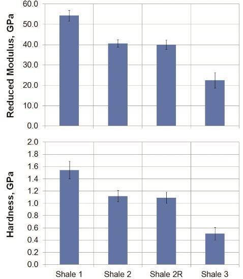
Figure 3. (a) Reduced modulus and (b) hardness of shale measured by instrumented indentation at 500mN. Each bar represents the mean of the eight median properties (one from each array) at 500mN. Error bars span the standard deviation of those eight medians.
The reported properties (Table 2, Figure 3) are repeatable and relevant. The results from the second round of testing on sample 2 are indistinguishable from those of the first round, thus lending credibility to the measurement technique and data-reduction process. Not surprisingly, the two samples from the Eagle Ford play had significantly different properties. This result highlights the importance of obtaining and testing samples for each well bore at all relevant depths.
Ion milling is an adequate method of surface preparation. There is no evidence that mechanical polishing confers a smoother surface for indentation testing. For all forces, the standard deviations in reduced modulus and hardness are about the same for the ion-milled samples as for the mechanically polished sample.
The constitutive properties obtained from the indentation results are summarized in Table 3, and the stress-strain curves corresponding to these properties are plotted in Figure 4. Only the Young’s modulus and yield stress are deduced from the indentation results. The Poisson’s ratio is assumed (ν = 0.25) as is the post-yield hardening (F = 0.01E).
Table 3. Constitutive properties for bilinear stress-strain curves, estimated from indentation measurements at 500mN. Stress-strain curves are plotted in Figure 4.
| Material |
E |
ν |
Y |
F |
| Shale 1 |
53.4 |
0.25 |
0.517 |
0.534 |
| Shale 2 |
39.5 |
0.25 |
0.373 |
0.395 |
| Shale 3 |
21.5 |
0.25 |
0.170 |
0.215 |
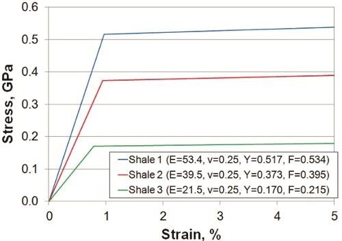
Figure 4. Stress-strain curves estimated from properties measured by instrumented indentation at 500mN.
The simulated force-displacement curves are plotted in Figure 5, together with typical experimental force-displacement curves (i.e., curves that happen to manifest properties close to those reported for the material as a whole at 500mN). The agreement is surprisingly good, given the complexity of the shale and the simplicity of the constitutive model. The bilinear stress-strain model with negligible hardening captures much of the mechanical behavior of the shale.
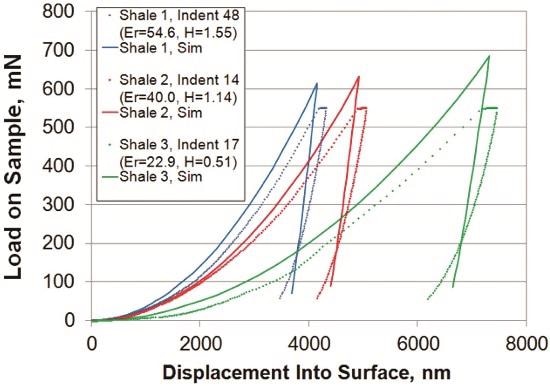
Figure 5. Simulated indentation curves, with test material modeled as having the stress-strain curves shown in Figure 4, compared with experiment indentation curves. Experimental curves were chosen (from among the 72 on each material) because they happened to manifest properties at 500mN that were very close to that of the bulk material.
The discrepancy between the simulated and experimental curves in Figure 4 is due primarily to creep. Creep is certainly occurring during the physical indentation test: during the 10-second dwell at 550mN, the indenter continues to progress more than 100nm further into the material. Although creep is most obvious during this dwell period, it is occurring throughout the test. However, our simple constitutive model does not have any mechanism for incorporating creep: all elastic and plastic deformation is assumed to be instantaneous. This is why, at any particular force, the experimental curve manifests a larger displacement than the simulated curve. In the experiment, the material is creeping, while in the simulation, it is not. Hence, the most fruitful improvement to the constitutive model would be the incorporation of time-dependent plasticity, wherein the yield stress, and thus the hardness, depend on strain rate and temperature in a predictable way. It is possible that the additional material properties required for such a constitutive model could also be measured by instrumented indentation.
The discrepancy between the simulated and experimental curves in Figure 4 is not due to the absence of significant work-hardening in our constitutive model. If we were to incorporate work-hardening into our constitutive model, the simulated curves would require an even greater force to achieve a particular displacement, and the discrepancy between simulation and experiment would be even larger. Hence, we are not motivated to improve the constitutive model by adding power-law hardening (like that often seen in metals) and trying to characterize such hardening by means of indenting with a spherical indenter. Work hardening is not something we must try to capture with our constitutive model, nor characterize by indentation.
Conclusions
Dynamic instrumented indentation is an ideal way to measure the mechanical properties of shale rock. Samples can be just a few millimeters in extent, and ion milling is an adequate method of surface preparation. For test forces greater than 300mN, the primary results (reduced modulus and hardness) are accurate, repeatable, and relevant. The bilinear stress-strain curves deduced from the indentation properties capture much of the mechanical behavior of the shale, as evidenced by good agreement between simulated and experimental indentation curves. The most fruitful improvement to the constitutive model would be the incorporation of creep.
References
[1] Sneddon, I.N., “The Relation Between Load and Penetration in the Axisymmetric Boussinesq Problem for a Punch of Arbitrary Profile,” Int. J. Eng. Sci. 3(1), 47–57, 1965.
[2] Pharr, G.M., Oliver, W.C., and Brotzen, F.R., “On the Generality of the Relationship among Contact Stiffness, Contact Area, and Elastic-Modulus during Indentation,” Journal of Materials Research 7(3), 613–617, 1992.
[3] Oliver, W.C. and Pharr, G.M., “An Improved Technique for Determining Hardness and Elastic-Modulus Using Load and Displacement Sensing Indentation Experiments,” Journal of Materials Research 7(6), 1564–1583, 1992.
[4] Hay, J.L., “Introduction to Instrumented Indentation Testing,” Experimental Techniques 33(6), 66–72, 2009.
[5] Hay, J.L., Agee, P., and Herbert, E.G., “Continuous Stiffness Measurement during Instrumented Indentation Testing,” Experimental Techniques 34(3), 86–94, 2010.
[6] Tabor, D., The Hardness of Metals, p. 37, 1951, London: Oxford University Press.
[7] Herbert, E.G., Pharr, G.M., Oliver, W.C., Lucas, B.N., and Hay, J.L., “On the Measurement of Stress-Strain Curves by Spherical Indentation,” Thin Solid Films 398, 331–335, 2001.
[8] Lucas, B.N. and Oliver, W.C., “Indentation Power-Law Creep of High-Purity Indium,” Metallurgical and Materials Transactions A - Physical Metallurgy and Materials Science 30(3), 601–610, 1999.
[9] Amin, K.E., Mukherjee, A.K., and Dorn, J.E., “A Universal Law for High-Temperature Diffusion Controlled Transient Creep,” Journal of the Mechanics and Physics of Solids 18(6), 413–426, 1970.
[10] ISO/FDIS ISO 14577-1:2002: “Metallic materials — Instrumented indentation test for hardness and materials parameters — Part 1: Test method.”
Nanomeasurement Systems from KLA
KLA offers high-precision, modular nanomeasurement solutions for research, industry, and education. Exceptional worldwide support is provided by experienced application scientists and technical service personnel. KLA's leading-edge R&D laboratories are dedicated to the timely introduction and optimization of innovative, easy-to-use nanomeasurement system technologies.

This information has been sourced, reviewed and adapted from materials provided by Nanomechanics, Inc.
For more information on this source, please visit Nanomechanics, Inc.